The Atlas Neuron

A neural network trained on one task and then on a second one forgets most of the first, so that a small network which learns 20 pixel-shuffled versions of MNIST one after another ends at 45% average accuracy, against 94% for the same network trained on all of them at once. This is usually addressed by replaying stored examples of earlier tasks or by slowing down the weights that mattered for them (Kirkpatrick et al., 2017).

The Atlas neuron keeps what it has learned by forking, i.e. it opens a new page whenever its inputs stop looking like any world it knows, and from then on only that page learns. On a page, every class is kept as typical examples (landmarks) together with a chart that consists of the class's mean and the 16 directions along which the class varies most. Every chart reconstructs the input from its mean and its directions, and a class is scored by how much its best chart leaves unexplained and by how similar the input is to its nearest landmark. Nothing is trained by backpropagation. The pages are built in one pass over the stream by online k-means and incremental PCA, with the two weights of the vote, which the neuron sets itself, as the only numbers learned by gradient descent.

At about the same memory as DER++ with 500 stored images (0.46M against 0.49M floats), the Atlas neuron is 5.3 and 4.5 points ahead of it on the two split benchmarks of the Mammoth continual-learning library, without task labels or replay. On the permuted benchmarks, where it stores 2.2 times as many floats as DER++ with 5,120 stored images, it leads by 4.4 to 20.0 points, and a lookup table built from twice as many of its own landmarks, which stores 42% more floats, is outperformed on five of the six benchmarks. The neuron's accuracy barely changes from the first to the hundredth world of a 100-world stream, and with a frozen feature layer learned without labels it can also be applied to natural images.

How an Atlas neuron works

Forking. Every image is compressed by a fixed random projection to 256 numbers, and the familiarity of a training batch is measured as the average similarity of its images to their nearest landmark, with the usual familiarity of a world measured over its first 50 batches and then frozen. The neuron is never told when the task changes, and a new page is forked for a new world after 3 consecutive batches below 85% of that usual familiarity (or when a batch shares no label with the current world and brings a label that no world has seen), with the batches of such a streak not learned from. Only the page of the current world learns, with the pages of all other worlds left exactly as they were, and a landmark stops moving after it has absorbed 1,000 images, which leaves slow drift (e.g. rotations a few degrees apart) to be noticed by the familiarity test and not absorbed step by step.

Landmarks and charts. For every class, a page keeps 128 landmarks in the 256-number code, updated by online k-means; the neuron recognises a world by them, and on their own they form a lookup table, i.e. a nearest-landmark classifier. The chart of a class, which is stored in pixel space, consists of the class's mean and the 16 directions along which its inputs vary most, and it is found by incremental PCA (Ross et al., 2008) as the images stream past, each of them seen once.

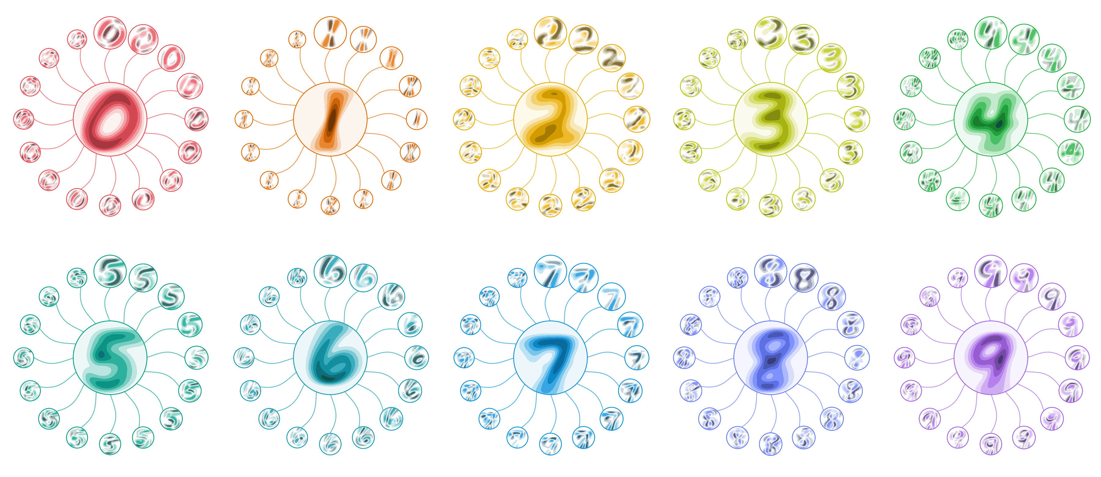Figure 2. Ten charts of one Atlas neuron (one per digit, each from a different world and drawn in that world's colour), with the chart's mean in the middle disc and its 16 directions as petals, starting at the top and going clockwise. Light and dark shades change the digit in opposite ways, and a petal is larger the more of the class's variation its direction explains.

As can be seen in Figure 3, each chart reconstructs an image by moving from its mean along its 16 directions to the point of its subspace closest to the image, and the squared distance left over is what the chart cannot explain. With its mean alone, a chart is a nearest-mean classifier, which here picks the 9, and from the third direction on the chart of the 4 comes closer to the input than that of the 9.

Loading the neuron (1.9 MB)…

The class score adds, with a weight for each, the smallest unexplained distance among the charts of the class and the similarity of its landmark closest to the input, both taken across all pages without routing the input to its world first.

Every world of Permuted MNIST shuffles the pixels in its own way, and the neuron, which never sees them in their original order, stores what looks like noise. With each pixel put back where its world took it from, 20 separately learned copies of the same ten digits appear (Figure 4).

What we found

The six benchmarks are run in Mammoth (Boschini et al., 2022), a widely used continual-learning library. The permuted benchmarks have 20 tasks, each with its own fixed shuffle of the pixels, and are built from MNIST or, with photos of clothing and handwritten Japanese characters, from Fashion-MNIST (Xiao et al., 2017) and KMNIST (Clanuwat et al., 2018). Rotated MNIST also has 20 tasks, in which every digit is turned by an angle drawn at random for its task, and Split MNIST and Split Fashion-MNIST bring two new classes in each of 5 tasks; all 10 classes must finally be told apart.

Every image is seen once, and we report the average test accuracy over all tasks after the last one, over 5 seeds. The baselines either restrict how weights change (online EWC, Kirkpatrick et al., 2017 and Schwarz et al., 2018; SI, Zenke et al., 2017; LwF, Li and Hoiem, 2017) or replay 200, 500 or 5,120 stored images (A-GEM, Chaudhry et al., 2019a; ER, Chaudhry et al., 2019b; DER and DER++, Buzzega et al., 2020). All of them use the small network of the DER paper (two hidden layers of 100 units) with its settings where it gives them, and our runs reproduce its numbers (88.1% for DER++ with 500 images on Permuted MNIST, against 88.2% reported). The lookup table consists of the Atlas neuron's own landmarks without its charts, and the Atlas neuron keeps 128 landmarks per class and 16 directions per chart, chosen on validation splits and never on test data.

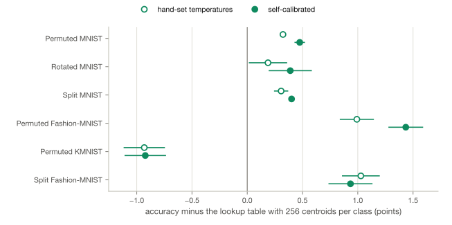Figure 5. Accuracy after the last task minus that of the lookup table with 256 centroids per class, as mean and standard deviation over 5 seeds of the difference between runs with the same seed. Open and filled circles are the Atlas neuron with hand-set temperatures and with its self-calibrated vote, respectively, and on every benchmark the Atlas neuron stores 70% of the lookup table's floats.

As can be seen in Figure 5, the Atlas neuron outperforms the lookup table with 256 centroids per class by 0.4 to 1.4 points on every benchmark except Permuted KMNIST, where it is 0.9 points behind, and on Permuted MNIST it reaches 96.7% against 96.2% with 9.2M instead of 13.1M floats. On Permuted MNIST, doubling the lookup table from 128 to 256 centroids per class gains 0.5 points for 6.6M more floats, and the charts, which are all that the Atlas neuron adds to its 128 landmarks, add more than these extra centroids (1.0 point for 2.7M floats).

How does replay compare at the same memory? DER++ with 500 stored images keeps about as many floats as the Atlas neuron on the split benchmarks (0.49M against 0.46M) and ends 5.3 and 4.5 points below it on Split MNIST and Split Fashion-MNIST, where DER++ with 5,120 stored images is behind as well (Table 1). On the permuted benchmarks, the Atlas neuron stores 9.2M floats, 2.2 times as many as DER++ with 5,120 stored images, and leads by 4.4 to 20.0 points, but replay was not run at that memory, and going from 500 to 5,120 stored images, i.e. to 8.5 times the memory, raises DER++ by 4.2 points on Permuted MNIST. On Rotated MNIST, DER++ with 5,120 stored images keeps three times as many floats as the Atlas neuron and ends 0.3 points ahead (94.5% against 94.2%).

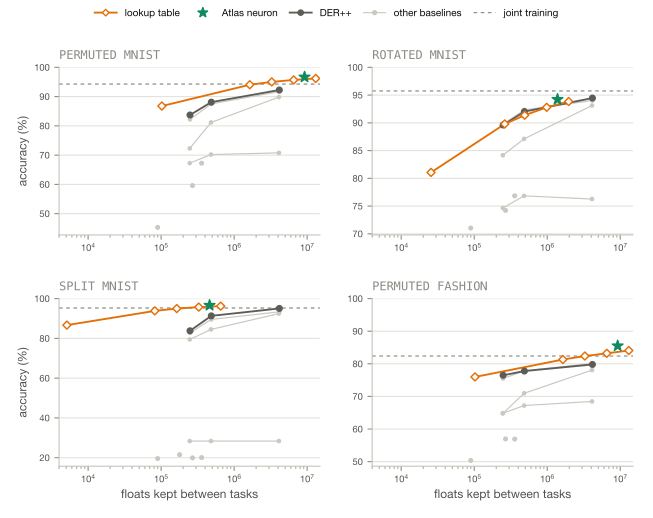Figure 6. Accuracy after the last task against the floats each method stores between tasks (log scale, means over 5 seeds) on four of the benchmarks. The Atlas neuron is the green star, and the lookup table with 4 to 256 centroids per class and DER++ with 200, 500 and 5,120 stored images are drawn in orange and dark grey, respectively, with the other baselines in light grey and joint training of the small network as a dashed line.

Full results (Table 1)

Average test accuracy (%) after the last task, mean ± standard deviation over 5 seeds, with the floats stored after the last task on the permuted benchmarks. The Atlas neuron and the lookup tables store less on Rotated MNIST, where the neuron finds 3 worlds on average, and on the split benchmarks (Atlas 1.38M and 0.46M, lookup with 256 centroids 1.97M and 0.66M, respectively).

Method	Floats	Permuted MNIST	Rotated MNIST	Split MNIST	Permuted Fashion	Permuted KMNIST	Split Fashion
Atlas, self-calibrated vote	9.22M	96.7 ± 0.0	94.2 ± 0.8	96.6 ± 0.0	85.5 ± 0.1	89.5 ± 0.4	85.0 ± 0.3
Atlas, hand-set temperatures	9.22M	96.5 ± 0.0	94.0 ± 0.8	96.5 ± 0.1	85.1 ± 0.1	89.5 ± 0.4	85.1 ± 0.2
Lookup, 256 centroids	13.11M	96.2 ± 0.0	93.8 ± 0.7	96.2 ± 0.0	84.1 ± 0.1	90.4 ± 0.2	84.1 ± 0.3
Lookup, 128 centroids	6.55M	95.7 ± 0.0	92.8 ± 0.8	95.7 ± 0.1	83.2 ± 0.1	89.0 ± 0.3	83.3 ± 0.3
DER++ (5,120)	4.16M	92.3 ± 0.1	94.5 ± 0.2	95.1 ± 0.3	79.8 ± 0.1	69.5 ± 0.3	81.8 ± 0.9
DER++ (500)	0.49M	88.1 ± 0.6	92.0 ± 1.1	91.3 ± 0.8	77.8 ± 0.1	63.1 ± 0.1	80.5 ± 0.6
Joint training (small network)	0.09M	94.3 ± 0.0	95.8 ± 0.2	95.3 ± 0.2	82.4 ± 0.2	75.7 ± 0.6	83.6 ± 0.9

A hundred worlds

On 100 permuted versions of MNIST, every world gets its own page, and memory grows with the number of worlds (with the hand-set temperatures). Against the lookup table with 64 centroids per class (95.0% at 16.4M floats), the Atlas neuron with 32 landmarks per class and 8 directions per chart ends at 95.2% with 15.3M floats, i.e. at about equal memory (Figure 7), and with 128 landmarks and 16 directions it reaches 96.5%, although it then stores 46.1M floats, 40% more than the lookup table with 128 centroids (95.7%). None of the curves in Figure 7 drops as the worlds arrive, while replay, which is not shown there, ends far behind (66.3% for ER and 73.9% for DER++ with 5,120 stored images).

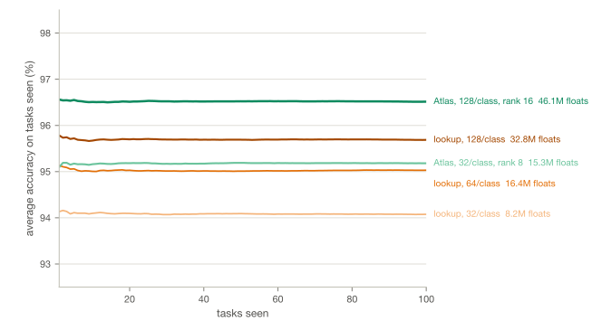Figure 7. Average accuracy over the worlds seen so far on 100 permuted versions of MNIST (mean over 3 seeds, test sets), with the floats each method stores after the last world.

A hundred worlds (Table 2)

Average accuracy (%) after the last of 100 tasks, mean ± standard deviation over 3 seeds, with the DER paper's Permuted MNIST settings for the replay baselines.

Method	Floats	Accuracy
ER (5,120)	4.11M	66.3 ± 0.3
DER++ (5,120)	4.16M	73.9 ± 0.5
Lookup, 32 centroids	8.19M	94.1 ± 0.1
Lookup, 64 centroids	16.38M	95.0 ± 0.0
Lookup, 128 centroids	32.77M	95.7 ± 0.0
Atlas, 32 landmarks, 8 directions	15.26M	95.2 ± 0.1
Atlas, 128 landmarks, 16 directions	46.11M	96.5 ± 0.0

A vote without hand-set weights

With hand-set temperatures, the two kinds of memory are combined by adding their log-probabilities, each divided by a temperature (0.02 for the landmarks and 5 for the charts, picked on validation data), although the second temperature is in pixel units and would have to be picked again for any new kind of input. In the self-calibrated vote, both are replaced by two weights learned during training, i.e. each training batch is first scored with the current pages, and the weights take one gradient step on how well this vote predicted the labels before the batch changes anything else. The weights start at the inverse of each part's spread across classes and so do not depend on the units of the input either (scaling every image by 100 gives the same predictions).

Calibration only uses images of classes whose chart in the current world has already been given at least four times as many images as it has directions. This leaves out the first batches after a new class or world arrives, which a chart built from only a few images explains badly and on which the vote would learn a low weight for the charts, and without it calibration cost up to 14 points on Split CIFAR-10 (49.2% against 63.4% with 256 directions per chart).

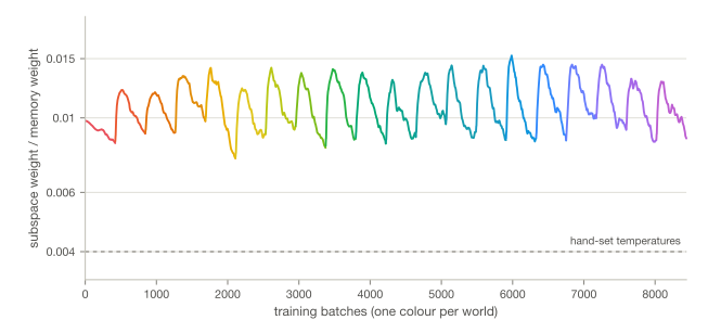Figure 8. Weight of the charts in the vote relative to that of the landmarks after every training batch on Permuted MNIST (log scale, coloured by world), which rises sharply soon after each new world arrives and decays as the world goes on, staying two to four times above the ratio implied by the hand-set temperatures (dashed) throughout.

As can be seen in Table 1, the self-calibrated vote does as well as the hand-set temperatures, with gains of 0.1 to 0.4 points on four benchmarks and differences of at most 0.1 points on the other two (a tie on Permuted KMNIST and 0.1 points less on Split Fashion-MNIST). Its learning rate barely matters, i.e. 0.003, 0.01 and 0.03 give the same validation accuracy to within 0.1 points on five benchmarks and to within 0.3 on Split Fashion-MNIST.

Natural images

Charts of raw pixels work for digits, which vary smoothly in pixel space, whereas on raw CIFAR pixels the Atlas neuron does poorly, as does every other method we ran (Krizhevsky, 2009; Table 3). For natural images it is therefore given a feature layer that is learned without labels or backpropagation in the style of Coates et al. (2011), in which every 6 × 6 patch of an image, normalised and whitened, is compared with 1,600 patch prototypes found by k-means, and each prototype responds in proportion to how much closer the patch is to it than on average to all prototypes. Pooling these responses over the four quadrants of the image gives 6,400 numbers, and the layer is learned from the first 1,000 images of the stream (on Split CIFAR-10 all aeroplanes and cars) and then frozen.

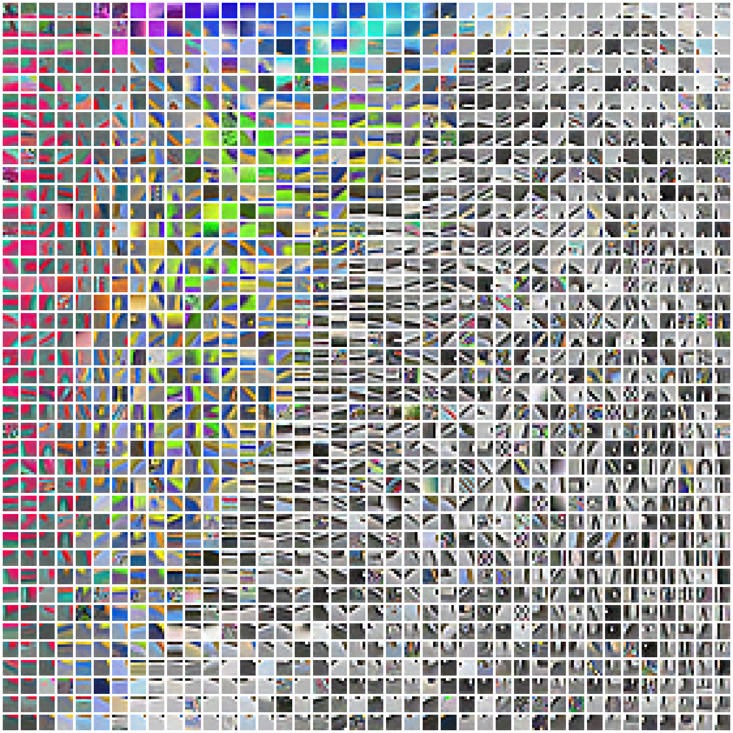Figure 9. The 1,600 patch prototypes of the feature layer, learned without labels from the first 1,000 images of Split CIFAR-10 and arranged so that similar prototypes are neighbours, with colour blobs and gradients on the left and oriented edges and corners on the right (each shown whitened and stretched to its own range).

As can be seen in Figure 10, the feature layer raises the Atlas neuron from 40.5% to 57.0% on Split CIFAR-10 and from 18.4% to 35.5% on Split CIFAR-100 (validation data, 3 seeds, every image seen once, no task labels), and streaming linear discriminant analysis (LDA; Hayes and Kanan, 2020) reaches more on the same features (77.2% and 50.1%, respectively). On these features, the covariance matrix that LDA shares across all classes (20.7M floats here) matters more than anything the per-class charts of the Atlas neuron capture. With only 256 directions of that covariance, LDA falls to 58.8%, about where the Atlas neuron is at the same memory, whereas above 2M floats, where LDA with its 1,024 strongest directions reaches 74.4% with 6.8M floats, the Atlas neuron is beaten at every memory size we tried.

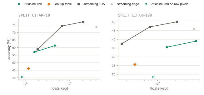Figure 10. Validation accuracy on Split CIFAR-10 and Split CIFAR-100 against floats stored (log scale, means over 3 seeds), all on the same frozen patch features except for the open circle, which is the Atlas neuron on raw pixels. The Atlas neuron with 16 and 64 directions per chart is drawn in green and streaming LDA in dark grey (with the shared covariance cut to 256 and 1,024 directions, and in full), while the lookup table with 128 centroids is orange and streaming ridge regression light grey.

Split CIFAR (Table 3)

Average validation accuracy (%) after the last task in the class-incremental setting with every image seen once, as mean over 3 seeds (standard deviations at most 0.9 points). Apart from the pixel rows, all methods use the same frozen patch features, whose 0.2M floats are included, and learning these features holds the first 1,000 images (3.1M floats) until the layer is frozen. The Atlas neuron uses the self-calibrated vote and 128 landmarks per class.

Method	CIFAR-10 floats	CIFAR-10	CIFAR-100 floats	CIFAR-100
Atlas, 16 directions, pixels	0.85M	40.5	8.50M	18.4
Lookup, 128 centroids, pixels	0.65M	34.5	3.60M	17.5
Streaming LDA, pixels	4.75M	39.4	5.03M	14.7
Atlas, 16 directions	1.61M	57.0	14.36M	35.5
Atlas, 64 directions	4.69M	61.4	45.08M	39.0
Lookup, 128 centroids	1.18M	46.1	4.13M	25.6
LDA, 256 directions	1.91M	58.8	2.48M	37.5
LDA, 1,024 directions	6.82M	74.4	7.40M	47.1
Streaming LDA	20.74M	77.2	21.32M	50.1
Streaming ridge regression	41.22M	73.6	41.80M	45.9

Related work

What should a learner do when its inputs stop looking familiar? Opening new memory in that case goes back to adaptive resonance theory (Carpenter and Grossberg, 1987), and continual learning has several variants of it, e.g. an expert added for every task and picked by the autoencoder that reconstructs the input best (Expert Gate; Aljundi et al., 2017) or new experts grown without task labels through a Dirichlet process mixture (CN-DPM; Lee et al., 2020). Of prior continual learners, iCaRL, which classifies by the nearest class mean of stored examples (Rebuffi et al., 2017), comes closest to the lookup table.

Classification by the class subspace that best explains the input is one of the oldest ideas in pattern recognition, with examples that range from the CLAFIC method of the 1960s and the subspace methods collected by Oja (1983) to Kohonen's adaptive-subspace self-organising map, which learns such subspaces online and competitively (Kohonen, 1996), and to the mixture of local linear models per class with which Hinton, Dayan and Revow (1997) recognised handwritten digits. Tangent distance compares a digit with prototypes that may be transformed slightly along directions known in advance (Simard et al., 1993), and for continual learning on frozen features, classes have been modelled by their own covariance (FeCAM; Goswami et al., 2023) or by one shared covariance (streaming LDA; Hayes and Kanan, 2020). A single page of an Atlas neuron, whose chart directions are learned from the stream, is close to the model of Hinton, Dayan and Revow, and the neuron combines such pages, forked per world without task labels, with landmarks and with a vote whose weights it sets itself, all learned in one pass without backpropagation.

Limitations and next steps

The Atlas neuron works on whatever features it is given, and raw pixels are enough on MNIST-sized images. On natural images, where a frozen patch layer learned without labels already lifts it by 16.5 points on Split CIFAR-10, neither a stronger feature layer nor charts that share directions across classes as LDA does have been tried yet. As in every method that keeps something for each world, memory and test-time cost grow with the number of worlds, and after 20 worlds scoring one image takes about 100 times the multiply-adds of the small network the baselines use, although on 100 worlds the Atlas neuron still beats the lookup table at about equal memory and its accuracy barely moves from the first world to the hundredth.

Worlds are detected from the inputs alone, without task labels, which finds every world whose inputs look different and merges nearby angles on Rotated MNIST, where the Atlas neuron still beats the lookup table. On the split benchmarks, new worlds are opened when new labels arrive, so these two benchmarks test the class memory of a page more than the detection of worlds. The lookup table stays ahead only on Permuted KMNIST (by 0.9 points, with 42% more floats), and the CIFAR results, unlike the test accuracies in Mammoth reported for the MNIST family, are validation accuracies from our own streaming harness. Comparisons with given world identities, with a single page, with forked versions of streaming LDA or per-class Gaussians and with replay at the Atlas neuron's memory are left to follow-up work.

References

• Aljundi, R., Chakravarty, P. and Tuytelaars, T. (2017). Expert Gate: lifelong learning with a network of experts. CVPR.
• Boschini, M., Bonicelli, L., Buzzega, P., Porrello, A. and Calderara, S. (2022). Class-incremental continual learning into the eXtended DER-verse. IEEE TPAMI.
• Buzzega, P., Boschini, M., Porrello, A., Abati, D. and Calderara, S. (2020). Dark experience for general continual learning: a strong, simple baseline. NeurIPS.
• Carpenter, G. A. and Grossberg, S. (1987). A massively parallel architecture for a self-organizing neural pattern recognition machine. Computer Vision, Graphics, and Image Processing 37.
• Chaudhry, A., Ranzato, M., Rohrbach, M. and Elhoseiny, M. (2019a). Efficient lifelong learning with A-GEM. ICLR.
• Chaudhry, A. et al. (2019b). On tiny episodic memories in continual learning. arXiv:1902.10486.
• Clanuwat, T. et al. (2018). Deep learning for classical Japanese literature. NeurIPS Workshop on Machine Learning for Creativity and Design.
• Coates, A., Ng, A. Y. and Lee, H. (2011). An analysis of single-layer networks in unsupervised feature learning. AISTATS.
• Goswami, D., Liu, Y., Twardowski, B. and van de Weijer, J. (2023). FeCAM: exploiting the heterogeneity of class distributions in exemplar-free continual learning. NeurIPS.
• Hayes, T. L. and Kanan, C. (2020). Lifelong machine learning with deep streaming linear discriminant analysis. CVPR Workshops.
• Hinton, G. E., Dayan, P. and Revow, M. (1997). Modeling the manifolds of images of handwritten digits. IEEE Transactions on Neural Networks 8(1).
• Kirkpatrick, J. et al. (2017). Overcoming catastrophic forgetting in neural networks. PNAS 114(13).
• Kohonen, T. (1996). Emergence of invariant-feature detectors in the adaptive-subspace self-organizing map. Biological Cybernetics 75(4).
• Krizhevsky, A. (2009). Learning multiple layers of features from tiny images. Technical report, University of Toronto.
• Lee, S., Ha, J., Zhang, D. and Kim, G. (2020). A neural Dirichlet process mixture model for task-free continual learning. ICLR.
• Li, Z. and Hoiem, D. (2017). Learning without forgetting. IEEE TPAMI 40(12).
• Oja, E. (1983). Subspace Methods of Pattern Recognition. Research Studies Press.
• Rebuffi, S.-A., Kolesnikov, A., Sperl, G. and Lampert, C. H. (2017). iCaRL: incremental classifier and representation learning. CVPR.
• Ross, D. A., Lim, J., Lin, R.-S. and Yang, M.-H. (2008). Incremental learning for robust visual tracking. International Journal of Computer Vision 77.
• Schwarz, J. et al. (2018). Progress & compress: a scalable framework for continual learning. ICML.
• Simard, P., LeCun, Y. and Denker, J. S. (1993). Efficient pattern recognition using a new transformation distance. NeurIPS.
• Xiao, H., Rasul, K. and Vollgraf, R. (2017). Fashion-MNIST: a novel image dataset for benchmarking machine learning algorithms. arXiv:1708.07747.
• Zenke, F., Poole, B. and Ganguli, S. (2017). Continual learning through synaptic intelligence. ICML.